


274 Agilent N5161A/62A/81A/82A/83A MXG Signal Generators User’s Guide
Custom Digital Modulation (Option 431)
Using Finite Impulse Response (FIR) Filters in ARB Custom Modulation
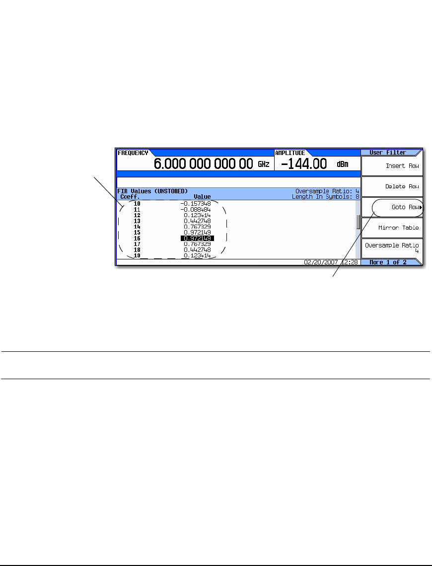
Duplicating the First 16 Coefficients Using Mirror Table
In a windowed sinc function filter, the second half of the coefficients are identical to the first half in
reverse order. The signal generator provides a mirror table function that automatically duplicates the
existing coefficient values in the reverse order.
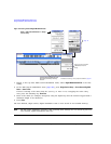
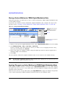
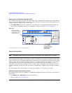
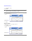
1. Press Mirror Table. The last 16 coefficients (16 through 31) are automatically generated and the
first of these coefficients (number 16) highlights, as shown in Figure 11-14 on page 274.
Figure 11-14
Setting the Oversample Ratio
NOTE Modulation filters must be real and have an oversample ratio (OSR) of two or greater.
The oversample ratio (OSR) is the number of filter coefficients per symbol. Acceptable values range
from 1 through 32; the maximum combination of symbols and oversampling ratio allowed by the table
editor is 1024. The instrument hardware, however, is actually limited to 32 symbols, an oversample
ratio between 4 and 16, and 512 coefficients. So if you enter more than 32 symbols or 512
coefficients, the instrument is unable to use the filter. If the oversample ratio is different from the
internal, optimally selected one, then the filter is automatically resampled to an optimal oversample
ratio.
For this example, the desired OSR is 4, which is the default, so no action is necessary.
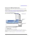
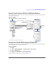
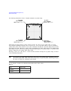
Displaying a Graphical Representation of the Filter
The signal generator has the capability of graphically displaying the filter in both time and frequency
dimensions.
1. Press More 1 of 2 > Display FFT (fast Fourier transform).
Refer to Figure 11- 15 on page 275.
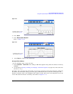
FIR table coefficient
values, may be from the
factory default values or
entered by the user.
Use the Goto Row
menu to move around
and make changes to
the FIR Values
coefficient table.
For details on each key, use key help as described on page 42.